
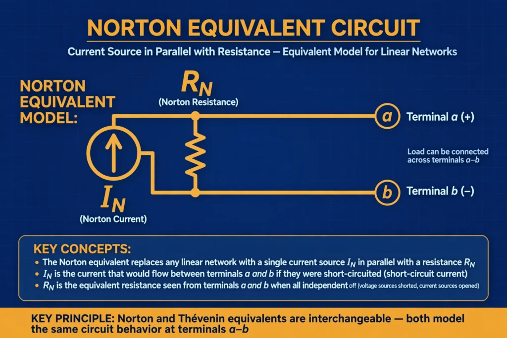

The Norton theorem is the current-source twin of the Thevenin equivalent: any linear network, seen from two terminals, can be replaced by one current source in parallel with one resistor. Where currents are the natural quantity — or current sources dominate — the Norton form is the more convenient choice.
Statement of Norton Theorem
Any linear bilateral network containing voltage sources, current sources, and resistors can be replaced by an equivalent circuit consisting of a single current source (IN, the Norton current) in parallel with a single resistance (RN, the Norton resistance), connected across the two terminals of interest.
The Norton current is the short-circuit current flowing between the two terminals when they are shorted together (with the load removed). The Norton resistance is found exactly the same way as the Thevenin resistance: turn off all independent sources and find the equivalent resistance seen from the terminals.
Once the equivalent is drawn, the load current follows from the current-divider rule: Load current = IN × RN / (RN + RL). Because the parallel equivalent behaves identically to the original network at the terminals, the load cannot tell the difference.
Step-by-Step Procedure to Apply Norton Theorem
Step 1: Identify the load and remove it
Choose the load branch (RL), remove it, and label the two open terminals A and B.
Step 2: Find the Norton current (IN)
Short-circuit terminals A and B and calculate the current flowing through that short. This short-circuit current is IN. (Do not actually short a live power circuit in practice — this is an analysis step for paper or simulation.)
Step 3: Find the Norton resistance (RN)
Turn off all independent sources: short-circuit voltage sources and open-circuit current sources. Then compute the equivalent resistance between A and B. This is RN, and it is numerically equal to Rth.
Step 4: Draw the equivalent circuit
Place the current source IN in parallel with RN, and connect the pair across terminals A and B.
Step 5: Reconnect the load and solve
Reconnect RL across A and B: IL = IN × RN / (RN + RL) by the current divider, and VL = IL × RL.
Quick reference table
| Quantity | How to find it |
|---|---|
| IN | Short-circuit current between A and B with load removed |
| RN | Equivalent resistance between A and B with sources turned off |
| Load current | IN × RN / (RN + RL) |
| Load voltage | IN × RN × RL / (RN + RL) |
| Relation to Thevenin | Vth = IN × RN, Rth = RN |
Solved Example 1: Norton Equivalent of a Two-Source Network
Take the same network as a classic teaching example: a 12 V source in series with a 4 Ω resistor, and a 3 Ω resistor from their junction to the reference node. The load RL = 6 Ω connects across the 3 Ω resistor (terminals A and B).
Step 1: Remove the 6 Ω load.
Step 2: Short terminals A and B. The short is in parallel with the 3 Ω resistor, so all current avoids the 3 Ω path and flows through the short. The current through the short is limited by the 4 Ω resistor in series with the 12 V source: IN = 12 V / 4 Ω = 3 A
Step 3: Short the 12 V source. From A and B, the 4 Ω and 3 Ω resistors are in parallel: RN = (4 × 3) / (4 + 3) = 12/7 ≈ 1.71 Ω
Step 4: The Norton equivalent is a 3 A current source in parallel with 1.71 Ω.
Step 5: Reconnect the 6 Ω load. Current divider: IL = 3 × 1.71 / (1.71 + 6) = 3 × 1.71 / 7.71 ≈ 0.667 A. Check against Thevenin: Vth = IN × RN = 3 × 1.71 = 5.14 V — matching the Thevenin result exactly, and the load current 0.667 A agrees as well. The two theorems always agree when done correctly.
Solved Example 2: Norton with a Current Source in the Network
Consider a network with a 5 A current source in parallel with a 10 Ω resistor, and a 20 Ω resistor also connected between the same two nodes. The load RL = 15 Ω connects across the node pair (terminals A and B). Find the load current.
Step 1: Remove the 15 Ω load, leaving open terminals A and B.
Step 2: Short A and B. The short sits directly across the current source and both resistors, so all 5 A flows through the short (a short has zero resistance, so it steals all the current): IN = 5 A
Step 3: Open-circuit the 5 A current source. From A and B, the 10 Ω and 20 Ω resistors are in parallel: RN = (10 × 20) / (10 + 20) = 200/30 ≈ 6.67 Ω
Step 4: The Norton equivalent is a 5 A source in parallel with 6.67 Ω.
Step 5: Reconnect the 15 Ω load: IL = 5 × 6.67 / (6.67 + 15) = 5 × 6.67 / 21.67 ≈ 1.54 A. Load voltage VL = 1.54 × 15 ≈ 23.1 V, and load power ≈ 35.5 W. Notice how natural the Norton form was here: with a current source in the network, IN fell out immediately.
Converting Between Norton and Thevenin
Because RN = Rth, conversion is a single step: IN = Vth / Rth takes you from Thevenin to Norton, and Vth = IN × RN takes you back. Choose the form that suits the problem: Thevenin when load voltage is the goal, Norton when current sources dominate or a current divider is cleaner.
Applications of Norton Theorem
- Circuits dominated by current sources: Transistor and sensor models are often current-source based, making the Norton form the natural choice.
- Parallel load analysis: When several loads sit in parallel across the same terminals, the Norton equivalent keeps the math in terms of currents, which add simply in parallel.
- Fault and protection studies: Short-circuit currents are the quantity of interest in protection design, and IN is literally a short-circuit current — the Norton form speaks the language of fault analysis directly.
- Simplifying before maximum power calculations: The Norton resistance is the same RN that determines the maximum-power load condition (see the maximum power transfer theorem).
- Two-port and active filter design: Norton equivalents of amplifier stages make cascading stages easy to analyze.
Limitations of Norton Theorem
- It applies only to linear networks — no diodes, no saturated transistors, no non-linear loads.
- It applies only to bilateral elements.
- Results are valid at the two terminals only; internal branch currents of the original network cannot be recovered from the equivalent.
- The “short the terminals” step is an analysis technique — never short-circuit a real powered network just to measure IN.
- Dependent sources need the test-source method to find RN, adding effort.
- Like Thevenin, it does not handle magnetic coupling across the terminal boundary or time-varying elements.
Relation to Other Circuit Theorems
Norton and the thevenin theorem are two faces of the same idea, converting with a single division or multiplication. The superposition theorem is often the easiest route to IN with several sources present. For background, see our guides to electrical symbols and the power triangle explained. Also see Wikipedia’s article on Norton’s theorem.
FAQs
What is the Norton theorem in simple words?
Any linear circuit, seen from two terminals, behaves exactly like a single current source in parallel with a single resistor. Find the short-circuit current (IN) and the resistance with sources off (RN), and you have the whole network in your pocket.
How is the Norton current found?
Remove the load, short the two terminals, and calculate the current through the short. That is IN.
Is Norton resistance the same as Thevenin resistance?
Yes. RN = Rth, always. Both are the equivalent resistance seen from the terminals with all independent sources turned off.
When should I use Norton instead of Thevenin?
Use Norton when the network contains current sources, when you are interested in short-circuit or fault currents, or when loads are in parallel and a current-divider form is cleaner.
Can Norton theorem be applied to AC circuits?
Yes. Replace RN with a complex impedance ZN and work with phasor currents — the steps are identical.
Why does the Norton equivalent use a current source in parallel?
Because the defining quantity IN is a short-circuit current. A current source in parallel with a resistor is the natural dual of Thevenin’s voltage source in series with a resistor, and both are exact representations of the same linear network.
Conclusion
The Norton theorem gives you the current-source dual of the Thevenin equivalent: one current source in parallel with one resistor captures everything a linear network presents at two terminals. The recipe — remove the load, find the short-circuit current, find the resistance with sources off, draw the parallel equivalent, reconnect the load — is short and reliable. Keep it paired with the thevenin theorem, reach for superposition when multiple sources make IN hard to see directly, and remember the limits: linear, bilateral networks, terminal behavior only.